
Friday, November 21, 2008
Tuesday, November 18, 2008
Define Profiles for the Projected Stock in SNC
Define Profiles for the Projected Stock
Use
In this Customizing activity, you define the following:
- Profiles for calculating the projected stock
- The projected stock is a key figure that indicates the available demand of a location product at the end of a day. It is calculated, application-specific, from actual stock on hand (+), demands (-), and receipts (+). Profiles for the projected stock are relevant for the following applications of SAP Supply Network Collaboration (SAP SNC):
- Supply Network Inventory (SNI)
- Replenishment Planning, for example in the SMI scenario or in the Responsive Replenishment scenario
- Delivery Control Monitor (DCM)
- For the DCM, only the stock on hand is relevant.
- Profiles for calculating the Demand key figure in SNI
- The Demand key figure specifies the demand of a location product at the end of a day. This profile is only relevant for SNI.
In the standard, the system uses preconfigured formulas to calculate the demand in SNI or the projected stock. Therefore, you only have to configure the Customizing activity in the following situations:
- You do not want to use the internal SAP default formula, but instead, you want to use your own formula as the default formula.
- You want to use different formulas for different business partner/location product combinations .
- Example for the SMI Monitor, in which the supplier plans the product requirements in the customer location: here you can use different formulas for different supplier/customer location product combinations.
Method for Calculating Projected Stock
In the standard, SAP SNC calculates the projected stock of a day using the following formula:
- Projected stock of a day = projected stock of the previous day + receipts with delivery date on that day - demands with demand date on that day
SAP SNC calculates the projected stock of today, that is, the initial projected stock, using the following formula:
- Projected stock of today = today's stock on hand + receipts with delivery date today - demands with demand date today.
The demands and receipts that the formula considers depend on the application. For example, the formula in the SMI Monitor considers the planned receipts and the stock in transit from issued ASNs. The stock types that are entered in the stock on hand are also application- dependent.
Consideration of Historical Values
For every key figure (receipt or demand), you can determine individually whether the system also considers the aggregated key figure values from the past when calculating the initial projected stock. Example: In Responsive Replenishment, you want to consider historical values of the Demand key figure in replenishment planning for promotions, but not in replenishment planning for baseline demand.
Default Formulas for Calculating Projected Stock
In the standard, the system considers the following key figures and stock types to calculate the projected stock:
- Projected stock for SNI
- The projected stock considers the stock on hand (+) and the following receipts and demands:
- Stock on hand (+)
- Planned receipts (+)
- Firm receipts (+)
- Demand (-)
- The demand includes the following demand types:
- Firm receipts
- Planned receipts
- Forecast demand
- Stock on hand includes the following stock types:
- Unrestricted stock
- The stock on hand is the same as the unrestricted stock.
- Projected stock for (baseline) replenishment in SMI and Responsive Replenishment
- The projected stock considers the stock on hand (+) and the following receipts and demands:
- Planned receipts (+)
- In-transit quantity (+)
- Demand (+)
- Stock on hand includes the following stock types:
- Unrestricted-use stock
- Unrestricted-use consignment stock
- Stock in quality inspection
- Consignment stock in quality inspection
- The DCM also considers these stock types for the stock on hand.
- Projected stock for promotion replenishment in Responsive Replenishment
- The projected stock considers the stock on hand (+) and the following receipts and demands:
- Planned receipts (+)
- In-transit quantity (+)
- Demand (+)
- Stock on hand includes the following stock types:
- Unrestricted-use stock
- Unrestricted-use promotion stock
- Stock in quality inspection
- Promotion stock in quality inspection
Stock on Hand
In the standard, the following stock types exist:
- Unrestricted-use stock
- Stock in quality inspection
- Locked stock
- The following consignment stock types:
- Unrestricted-use consignment stock
- Locked consignment stock
- Consignment stock in quality inspection
- The stock type that is considered by the internal default formulas for the stock on hand depends on the application. For more information, see the Default Formulas for Calculating Projected Stock section (see above). The stock on hand is calculated by the default implementation of the BAdI /SCA/ICH_STOCKONHAND. If required, you can use the BAdI to implement your own procedure for calculating the stock on hand.
Calculation of the Demand Key Figure for SNI
In the standard, the Demand key figure in SNI includes the following demands:
- Firm receipts (for example, from sales orders or production orders)
- Planned receipts (for example, from planned orders)
- Forecast demand
You can define your own formula. In addition, you specify the start and end of the horizon for which a formula is valid. In this way, you can define multiple subsequent horizons, in which the system uses a separate formula in each to calculate the demand. Example: in the short-term horizon, you only consider firm receipts, in the medium-term horizon you consider firm and planned receipts, and in the long-term horizon you only consider forecast demands.
Definition of Own Formulas
In your own profile, you can consider your own formula with any stock types and key figure. Beware of the following:
- Terms of the key figure type can be entered in the formula with either a positive or a negative sign.
- Terms of the stock type type must always have a positive sign.
Activities
- 1. If you want to work with your own formulas for the Demand key figure in SNI or for the projected stock, create a profile. To do so, define the following for each term that you want to include in the formula: an entry consisting of the profile name and the name of the term.
- 2. Define the sign for the term and the term type.
- 3. Select the profile as the standard profile for a specific application, if required. If you do not select any profile as the standard profile, SAP SNC uses the SAP standard formula (see above).
If you want to use different formulas for different business partner/ /location product combinations, create a profile for each required formula. In the Customizing activity Assign Settings for Replenishment Planning and SNI, you then assign the profiles to the required characteristics combinations.
Example
Wednesday, November 12, 2008
Note 546079 - FAQ: Background jobs in Demand Planning
Summary
Symptom
This note contains frequently asked questions/answers on the subject of
the mass processing in Demannd Planning
FAQ, Q+A, /SAPAPO/MC8D, /SAPAPO/MC8E, /SAPAPO/MC8F, /SAPAPO/MC8G,
/SAPAPO/MC8K, /SAPAPO/MC90, SM37
QUESTIONS OVERVIEW
Q1: How should I define an "Aggregational level" in background job?
Q2: What should I put in a "Selection" field in background job?
Q3: Why can I observe a "difference" in results of interactive planning and background job?
Q4: How can I increase performance of the background job?
Q5: How should I define a macro in background job?
Q6: How should I define a release of planned demand to SNP in background job?
Q7: How should I define a transfer of planned demand to R/3 in background job?
QUESTIONS & ANSWERS
Q1: How should I define an "Aggregation level" in background job?
A1: Select the characteristics that correspond to the aggregation
level on which you want the job to be carried out. The aggregation
level can make a big difference to the job results. When you run
the job at aggregated level (eg. you want to run a forecast
for a Sales Organization -> aggregation level = Sales Organisation)
only the aggregated data of the Sales Org. will be taken for the
forecast and than the forecast will be disaggregated to the
detailed level (eg. products) according to your aggregation/
disaggregation method defined for each key figure during definition
of planning area.
Use navigational attribues in selection and aggregation level when
you what to restrict processed data without implicit using of
characteristics.
Do not select characteristics which are not included in a
Selection for which you run the job.
For additional information please refer to the note 374681
and to online documentation (http://help.sap.com)
Q2: What should I put in a "Selection" field in background job?
A2: You can run the job for the characteristic value combinations in a
selection(s) you created earlier in the Shuffler (Interactive
Demand Planning). It is advisable to select value(s) for the
characteristic which was meant as display characteristic in the
selection.
Q3: Why can I observe a "difference" in results of Interactive Planning
and background job?
A3: There are several issues which can make you think that there are
differencies between online and batch results.
1) The selection you entered along with the aggregation level
are used as a basis for the individual, dynamically created
selections(!), which are used for calling the forecast.
In interactive planing, the selection is used directly for the
forecast. Consequently, you might be comparing the results from
different selections.
Example:
You want to do forecast for product A. The forecasting method
is defined as HISTORY + 1 = FUTURE.
Your selection consist of 3 characteristics:
1) Sales Org. 1000
2) Division, 01 02
3) Product A B A B
History (detailed level): 10 20 30 40
The online forecast for product A looks like:
(10+30) + 1 = 41(!)
In background job with the aggregation level Sales Org., Division
and Product the forecast will be done for 2 combinations:
[10 + 1 = 11] + [30 + 1 = 31] = 42(!)
2) In both cases (online and batch) the system uses
the corrected history for the calculation of the forecast.
During batch processing the system does not save the values
for corrected history if the planning book definition for this key
figure is 'not ready for input'. During interactive planning the
system allows to save the data in this line of the planning book.
For additional info please refer to notes 357789, 372939
and to online documentation (http://help.sap.com)
Q4: How can I increase a performance of background job?
A4: Because you generally do not need all data of the planning area and
because in general you need different data for different planning
processes, please maintain a specific planning book and data view
for your background job. The planning book should consist only of
the key figures which are necessary, and the time buckets in data
view should be restricted to the date you need for the job.
Horizon of the planning book must be greater than the horizons in
the forecast profile.
The time period units of the planning book and forecast profile
must be identical because you are not allowed to use planning books
with mixed period units in the background processing (note 357789).
If you set Generate log indicator for your jobs you have to delete
the log periodically. If you do not do this, performance will
deteriorate noticeably! You should regulary use the transaction
/SAPAPO/MC8K (Demand Planning -> PLanning -> Demand Planning in
Background -> Delete Job Log (note 512184). You can easily check
the size of the log by checking the table /SAPAPO/LISLOG.
For some cases (e.g. loading planning areas) you can divide a job
in smaller parts (new jobs) and run it in parallel. The same
objects cannot be processed by the parallel processes (locking
problems). There must be a separation using suitable selection
restrictions in the characteristics combinations (note 428102)
Q5: How should I define a macro in background job?
A5: Before you execute your own macro in the job, you must make sure
that you have implemented all macros that provide your own macro
with data. You must remember that standard macros in Interactive
Planning (start, level and default macro) are not automatically
executed in background job. You must choose proper aggregation
level with data to be changed by the macro.
You define an activity to run a macro for background job with
transaction SAP menu -> Demand Planning -> Environment ->
Current Settings -> Define Activities for Mass Processing
When a macro run didn't change a value (the same value already
existed) you will of course not need to store any data either.
For this reason, the message "Data were stored" will not appear
in the log. In other words, the message "Data were stored" will
only appear if new data have in fact been saved.
For additional info please refer to note 412429.
Q6: How should I define a release of planned demand to SNP in
background job?
A6: You should define an activity and a release profile (/SAPAPO/MC8S)
for mass processing to release a demand from DP to SNP.
The period of the release is defined by future and history time
time buckets profile maintained in the used dataview.
When you want to release data with offset periods you have to use
BAdI /SAPAPO/SDP_RELDATA bacause offset field of the dataview
is not taken into account for release!
After every release all SNP data of the product in the location
are deleted and only the just released data exist in SNP afterwards
You define the periodicity of the release (e.g. weeks, months) with
time buckets profile used in the dataview. When your time bucket
consist of 2 weeks and 3 months and when the time bucket is used
as history bucket and future bucket your data will be released in
this way:
M3 M2 M1 W2 W1 today W1 W2 M1 M2 M3
For additional info please refer to note 403050.
[online you can use trx: /SAPAPO/MC90 or report
/SAPAPO/RTSOUTPUT_FCST, only for small number of data(!)]
Q7: How should I define a transfer of planned demand to R/3 in
background job?
A7: You should define an activity and transfer profile (/SAPAPO/MC8U)
for mass processing to release a demand from APO DP to R/3. The
Requirements Type determines the planning strategy to be used for a
material requirement in R/3 (e.g. VSE "Planning w/o final assembly"
or VSF "Planning with final assembly"). It is not possible to
transport and save PIR on R/3 side without requirements type.
The requirements type must be transported from APO or if it is not
filled on APO side, then it must be customized on R/3 side
(material master). If you transport forecast from APO to R/3, data
on both sides must
be consistent after transport -> all transported PIR must be saved
on R/3 side or stay in outbound (inbound) queue.
When you want to change data before transfer you can use
BAdI /SAPAPO/IF_EX_SDP_RELDATA.
[You can use trx /sapapo/dmp2 to transfer data from SNP to R/3]
Header Data
| Release Status: | Released for Customer |
| Released on: | 13.02.2003 17:42:47 |
| Priority: | Recommendations/additional info |
| Category: | FAQ |
| Primary Component: | SCM-APO-FCS-MAP Mass Processing |
| Secondary Components: | SCM-APO-FCS Demand Planning |
| SCM-APO-FCS-MAC MacroBuilder |
Affected Releases
|
Related Notes
Tuesday, November 11, 2008
Maintaining Master Data for Scheduling Agreements (SMI)
In the SAP backend system, you maintain master data for a scheduling agreement because
gross demands for Supplier Managed Inventory (SMI) will be created based on this
scheduling agreement. This scheduling agreement is needed as basis for the goods receipt
posting and therefore as link for posting to accounts. Other process steps are built upon this,
such as invoice verification.
As there is no planning run that can create scheduling line items automatically (if
material is excluded from MRP), users have to maintain a “dummy” scheduling
line, otherwise goods receipt postings would be rejected.
Monday, November 10, 2008
Note 488725 - FAQ: Temporary quantity assignments in Global ATP
Note 488725 - FAQ: Temporary quantity assignments in Global ATP
Summary
Symptom
This note contains frequently asked questions on the subject of
'Temporary/persistent quantity assignments in Global ATP'.
CAUTION: This note is updated regularly.
- 1. What are temporary quantity assignments and why are they necessary?
Temporary quantity assignments reserve (or lock) quantities allotted during an ATP check in APO against opposing parallel ATP checks. The quantities remain locked until the order which triggered the ATP check is either saved or exited without saving. In either case, the related temporary quantity assignments are deleted. In the first case, they are no longer required because the order was cancelled, while in the second case, the updated order reserves the quantities itself in APO. A separate quantity assignment is then no longer necessary. This means that temporary quantity assignments exist only for the short duration of a transaction. An exception to this rule is the case of persistent quantity assignments (see FAQ point 2), which are still present after the end of an transaction. Quantity assignments are stored in the liveCache and once they are created, they are immediately displayed for all parallel transactions. You can identify temporary quantity assignments in the monitor (transaction /SAPAPO/AC 06) by the persistency indicator N (= non-persistent). All ATP basic methods (product availability check, product allocation, check against planning) create their own temporary quantity assignment.
- 2. What are persistent quantity assignments?
Unlike temporary quantity assignments, persistent quantity assignments continue to exist after a transaction is ended, that is, they reserve quantities over a longer, unspecified period until they are deleted by another transaction. The persistence indicator for persistent quantity assignments changes depending on the transaction phase they are in: In the transaction that creates them, they have the indicator V
(= prepersistent), and when the transaction is exited with 'Save', they are assigned the indicator P (= persistent), otherwise they are deleted. If another transaction has read or downloaded the persistent quantity assignments, they acquire the indicator O (= postpersistent). If this downloading transaction is then saved (updated), the postpersistent quantity assignments are deleted.
Persistent quantity assignments are used in the following scenarios:
- Backorder processing (batch with postprocessing and interactive operation)
- ALE third-party order processing ( 'old third-party')
- CRM scenario ('old' CRM scenario where the requirements are contained in R/3, not in CRM)
- Multi-level ATP check (as of APO 3.1)
The following section recaps the transition between the various persistence indicators, using the example of backorder processing:
During backorder processing, prepersistent quantity assignments are written as a result of the checks. When the backorder processing is then saved, the quantity assignments become persistent (the 'Backorder processing' transaction is thus completed). If this backorder processing is to be updated, the results are sent to R/3, updated there and then sent to APO using the core interface (CIF). In APO, the related quantity assignments are now imported by means of the update transaction and switched to postpersistent. Once the update is complete, the postpersistent quantity assignments are deleted. The postpersistent status is required to allow postpersistent quantity assignments to be switched back to persistent in the event of an error (that is, if the APO update encounters an error and is not committed). If the assignments are already deleted, they can no longer be restored.
- 3. What are quantity assignments of the type 'Advanced Planning and Scheduling'?
These quantity assignments, also known as APS delta records, differ fundamentally from the temporary and persistent quantity assignments described above. The main difference is that APS delta records are not quantity assignments, but time series entries for temporary planned orders. They are used in the CTP (Capable-To-Promise) scenario. In this scenario, temporary planned orders may sometimes be created during the ATP check and updated in the order network in the liveCache. However, the planned orders are not yet contained in the ATP time series in the liveCache since they could then be read by parallel ATP checks and used for confirmation. Therefore, instead of temporary planned orders being entered in the ATP time series, APS delta records are created for the planned orders. Once the CTP check result is saved and the temporary planned order becomes a 'real' planned order, the APS delta records are entered (incorporated) in the ATP time series. Otherwise, the APS delta records are simply deleted. Three APS delta records are created for each temporary planned order:
One for 1.1.1970 with quantity -X
One for 1.1.1970 with quantity -X
One for the correct date of the planned order with quantity X
The reason for the peculiar records for 1.1.1970 is explained by the method of operation of the scheduler in the liveCache order network. The receipts are always first created on 1.1.1970 (which is time 0 in the UNIX environment) and are then moved to the correct time.
Report /SAPAPO/OM_DELTA_COMPRESS compresses the delta records (for example, it deletes unnecessary delta records for 1.1.1970) and should always be executed if there are many delta records and you want a clear overview.
You can display APS delta records with the display function for temporary quantity assignments. For this purpose, select the relevant category 'Advanced Planning and Scheduling' and leave the User field blank. APS delta records are always written with the system user 'THE_NET'.
APS delta records should not be deleted manually since this can cause inconsistencies in the ATP time series. In any case, remaining delta records are not problematic because they do not reserve quantities. However, you must be careful when manually deleting temporary planned orders. You should only do so using the standard product heuristics in the product view, since in this case the related APS delta records are incorporated in the ATP time series. If you do not use the standard product heuristics, negative ATP time series entries can result, because the corresponding quantity is subtracted from the ATP time series as a result of deleting the planned order (even though the quantities were not contained in the ATP time series because there are only APS delta records). If these inconsistencies have occurred, you can incorporate the APS delta records subsequently using report /SAPAPO/ATP_SERVICE. To do this, simply select the product and location in the report and then select the option for incorporating delta records. The corresponding APS delta records then disappear and the ATP time series are consistent again.
After you implement Note 970113 (SCM 4.1 and higher), CTP and GATP are integrated to such an extent that APS delta records are no longer necessary.
- 4. Why is
- 5. This happens if the order number is (still) unknown when the quantity assignment is created. In fact, since this is the usual scenario for temporary quantity assignments, it is NOT an error.
For example: A sales order is created in R/3 and checked in APO. The check generates non-persistent quantity assignments with an unknown order number because this order does not yet exist in APO. The order only exists in APO after the order is saved in R/3, posted and then transferred to the APO via CIF. However, the temporary quantity assignments are already gone (they are deleted immediately after the APO posting). This means that these non-persistent quantity assignments can never have an order number.
The order number field is for information purposes only and is not a key field for the quantity assignments. As a result, even though in theory it would be possible, the order number is not added subsequently when the persistent delta records are posted either.
- 6. Sometimes quantity assignments with product or location 'PeggingID not found' appear in the display of the temporary quantity assignments (transaction /SAPAPO/AC06). Why is this? Can these quantity assignments be deleted?
Every product location combination (or pegging area) is encrypted by a GUID. This pegging area is usually in the liveCache and on the APO database. The quantity assignments display determines the temporary quantity assignments from the liveCache and then tries to convert the GUID of the pegging area into readable product and location names. The conversion is performed by reading the pegging area data on the database. If this entry is not found on the database, 'PeggingID not found' is displayed as product and location. One reason for this may be inconsistencies between the liveCache and database - the pegging area may be in the liveCache, but not in the database. You can use transaction /SAPAPO/OM17 to eliminate these inconsistencies. Pegging areas are frequently missing in the case of make-to-order production because these are created dynamically and deleted.
The quantity assignments with unknown pegging area should first be regarded as normal quantity assignments (they can be deleted if old and no longer required).
- 7. Why are no quantity assignments displayed in the display of the temporary quantity assignments (transaction /SAPAPO/AC06), even though * was entered as a user?
No wildcards can be used in the user selection. To display temporary quantity assignments for all users, leave the user field blank.
- 8. Why are quantity assignments left even though they should have already been deleted? What is the cause and how can the quantity assignments be deleted?
Sometimes, quantity assignments are not be deleted. There are many reasons for this, depending on the particular scenario used. There is therefore no generally applicable procedure for determining why quantity assignments remain. The following section gives some tips on eliminating problems with remaining quantity assignments (depending on the given scenario).
- General information
In most cases, quantity assignments are deleted using the CIF interface, depending on activities in R/3 (such as saving/terminating an order, posting backorder processing). The related queue entries (transaction SMQ1 in R/3 or SMQ2 in APO if you switched to inbound queues) start with CFTG, followed by a GUID. These queues contain the /SAPAPO/CIF_GEN_TID_INBOUND module, which is responsible for deleting quantity assignments. Therefore, if quantity assignments remain, you should first check whether there are corresponding queue entries. If so, these must be restarted. You should never delete the queues, because then the system does not delete the related quantity assignments and you must therefore eliminate them manually. If no queue entries are present, you can use transaction SM58 (Selection with initial user) to check in APO if there are entries of the module /SAPAPO/DM_DELTA_CLEAR_TRGUID. This module is responsible for deleting the quantity assignments in APO. Any entries found must be processed. Since locking problems are often the reason why these entries are left, you should check transaction SM58 regularly and process it if necessary. This transaction can be scheduled as a batch job by scheduling report RSARFCEX as a job. In this case too, the entries must never be deleted, since otherwise the related quantity assignments are no longer deleted.
- Backorder processing
Prepersistent quantity assignments are written during backorder processing and these become persistent after saving. These remain until backorder processing is posted or deleted. They are posted on an order-by-order basis, that is, while the orders involved are posted in APO, the related persistent quantity assignments change to postpersistent and then the postpersistent quantity assignments are deleted via the CIF queue. If persistent quantity assignments of a posted backorder processing remain, you should check whether backorder processing was actually fully updated afterwards in APO (status 'X' = update ended). It is possible that not all quantity assignments are deleted immediately when data is updated afterwards in APO, but only when the last order is transferred (when backorder processing has the status 'Update ended' ). An overall deletion call then takes place for all remaining quantity assignments of this backorder processing.
In this regard, it should be mentioned that a quantity assignment cannot always be assigned precisely to an order item with the POSGUID in backorder processing. The reason for this is that quantity assignments during the backorder processing checks are only written if the cumulative confirmed quantities exceed the quantities already confirmed before the backorder processing. In calculating whether this limit (high-water mark) of already confirmed quantities is exceeded, the assignment to the order item list is lost - this means that a quantity assignment may sometimes be written for an order item, even though a quantity was no longer assigned to it by backorder processing. This does not affect the system, as only the sum of the locked quantities is important. However, the system response can cause some confusion, particularly if quantity assignments were not deleted completely after backorder processing.
- ALE third-party order processing / CRM scenario
In these scenarios, prepersistent quantity assignments are written during the online ATP check, and are then converted to persistent quantity assignments when the order is saved. These remain until the order is transferred to the connected second OLTP System and updated there. If persistent quantity assignments now remain, you should check whether the transferred order has a confirmed quantity. If not, the previous confirmation from the first R/3 or CRM system could not be assigned to the transferred order. This is often due to the first and second system having different settings for transport and shipping scheduling. If this is not the case, you should check the queues (as described under general information), in both the first and the second system.
If you cannot determine and eliminate the cause of the remaining quantity assignments, you can delete them manually. You can do this using the monitor for temporary quantity assignments (transaction /SAPAPO/AC 06). You can select quantity assignments on the display screen and delete them by choosing Delete (the garbage can with text 'TrGuid'). This deletes all quantity assignments that were written by the system in the same transaction (that is, all assignments with the same transaction GUID). For this reason, all you have to do to delete all quantity assignments for a backorder processing run is select a single quantity assignment since all quantity assignments for this backorder processing have the same transaction guid.
In addition to this manual deletion procedure, you can also use the deletion report /SAPAPO/OM_DELTA_REMOVE_OLDER. This report deletes all selected quantity assignments, depending on how old the quantity assignments are and on the user who created the quantity assignments. Of course, you can also use transaction SM36 or SM37 to schedule the report as a batch job and then regularly delete old quantity assignments. However, in this case, you must be careful not to delete quantity assignments that are still required. These vary according to customer and the scenario used. Non-persistent quantity assignments that are older than a day can usually be deleted since these are only supposed to exist for a very short time. In the case of persistent quantity assignments, it depends on how long the overall process takes (for example, the maximum time needed to update a backorder processing run). If a customer frequently has backorder processing that is only updated after 3 days, no persistent quantity assignments younger than 3 days should be deleted.
- 9. Why are quantity assignments not deleted automatically during a rollback? I want to understand the technical background and potential problems that may occur when I delete quantity assignments.
Naming the function modules that are not released is simply a debugging tool. It does not mean that SAP allows you to use these modules in your own applications. As of SCM 4.1, SAP offers released function modules with the same functions in the same function group but that are not used by SAP-specific programs.
The temporary quantity assignments are written to the liveCache using a second database connection and are committed immediately. This ensures that they are immediately visible for parallel transactions but this also means that they are not automatically deleted during a rollback. The "task handler" is available for an almost automatic deletion of quantity assignments. The task handler is triggered as soon as the RFC connection between the calling system and the SCM is (unexpectedly) ended. It deletes all quantity assignments written in the transaction, but it cannot recuperate the non-persistent quantity assignments that were implicitly deleted in the transaction. Terminations that do not break off the RFC connection (for example a dump in the SAP GUI) cannot be caught by the SCM system.
Once a transaction is terminated successfully, the task handler must be deregistered. This is done by calling either "BAPI_APOATP_INITIALIZE" or "BAPI_APO_TASKHANDLE_DEREGISTER". Any terminations in the calling transaction after this event cannot be caught by the SCM system.
The calling transaction is also responsible for removing the relevant quantity assignments again. If the transaction terminated successfully, this can be done either by calling "/SAPAPO/CIF_GEN_TID_INBOUND" using CIF or "BAPI_APOATP_REMOVE_TMP_OBJECTS" directly using RFC. If there is a late rollback (for example because of an update termination) the deletion can only take place using "BAPI_APOATP_REMOVE_TMP_OBJECTS".
Up to SCM 4. 1, the attempt to delete quantity assignments may fail if the anchor object of the quantity assignment in the liveCache is currently locked by another transaction. A failed deletion attempt by the task handler cannot be repeated. A failed deletion attempt using CIF ensures that a tRFC hangs with the status "errors" and this can be restarted manually using transaction SM58 or automatically by report ???. A failed deletion attempt using "BAPI_APOATP_REMOVE_TMP_OBJECTS" returns an error message to the calling application.
- 10. What technical changes have been made to quantity assignments between releases and why?
Up to and including SCM 4. 0, temporary quantity assignments were also protected by an enqueue lock on the anchor object. Since, for technical reasons, the task handler cannot consider an enqueue lock, and since it can be very difficult to get simultaneous locks for all anchors in documents with many items, as of SCM 4.1 (Note 780510), we have removed the enqueue lock for temporary quantity assignments in the product availability check.
Instead, we introduced a repeat mechanism which allows for a repeated partial deletion. This repeat mechanism has only been used efficiently in the CIF call since Note 960279 (SCM 4.1) or 813546 (lower releases).
In SCM 5.0 the administration objects in the liveCache are completely parallel, with the result that a technical lock in the liveCache is no longer possible.
- 11. What are active, passive and aggregated quantity assignments?
As part of the multi-level ATP check for APO 3.1, a new status for quantity assignments was introduced, which is referred to as the type of a quantity assignment. There are four different types in total: active, preactive, passive and prepassive quantity assignments.
- Active quantity assignments are those assignments used up to and including APO 3.0, in other words, quantity assignments known to date.
- Passive quantity assignments are required for reservations at component level (dependent requirements) in the multi-level ATP check. All passive quantity assignments are aggregated and available as aggregated quantity assignments in the liveCache. These aggregated quantity assignments are read by parallel checks and they reserve the necessary requirements and confirmations at component level. The passive quantity assignments themselves no longer reserve any quantities, but exist for information purposes only, since their aggregates lock. Hence the name 'passive'. They are deleted if the ATP tree structures generated by the multi-level ATP check is converted to PPDS planning objects.
- Prepassive quantity assignments are written online for the components during the multi-level ATP check. When the order is saved, they are converted into passive quantity assignments and aggregated. Prepassive quantity assignment have an 'active' function, in that they do reserve quantities, unlike the passive quantity assignments described above.
- Preactive quantity assignment are written online during the multi-level ATP check and converted into active quantity assignments when the order is saved. While they have a 'passive' nature because they do not reserve any quantities themselves, they are not aggregated. Preactive quantity assignments are required to release any excess quantity locked by the order at the final material level, so they are always preceeded with a minus sign.
For example: A sales order for 100 pieces of a final material is created and checked at several levels. At the final material level, 40 pieces are confirmed directly by stock, while the remaining 60 can be produced. The customer requirement now receives the entire confirmation of 100 for the final material and is thus updated as such when saved. However, this means that the sales order reserves 100 pieces of the final material itself, which is incorrect because only 40 were confirmed at the final material level and only these may be reserved. For this reason, a preactive quantity assignment for -60 is written for the final material. As a result, only the total of 40 pieces is locked for parallel checks.
- 12. Why are the quantity assignments inconsistent and incorrect after a liveCache crash followed by a liveCache recovery? How can the inconsistencies be eliminated?
This can only occur with APO 3.0 and a liveCache version lower than 7.4. Note 435827 provides a detailed description of the causes and the procedure for cleaning up the inconsistencies.
As of liveCache Version 7.4, the liveCache handles data backup and recovery, so errors of this type should no longer occur.
-
Header Data
| Release Status: | Released for Customer | |||||||||||||||||||||||||||||||||||||||||||||||||||||||||||||||||||||||
| Released on: | 02.10.2006 18:15:26 | |||||||||||||||||||||||||||||||||||||||||||||||||||||||||||||||||||||||
| Priority: | Recommendations/additional info | |||||||||||||||||||||||||||||||||||||||||||||||||||||||||||||||||||||||
| Category: | FAQ | |||||||||||||||||||||||||||||||||||||||||||||||||||||||||||||||||||||||
| Primary Component: | SCM-APO-ATP Global Available-to-Promise Affected Releases
Related Notes
|
Monday, November 3, 2008
Beginner’s Guide to ALE and IDocs
Source: http://www.riyaz.net/blog/beginners-guide-to-ale-and-idocs-a-step-by-step-approach
In the previous parts we learned how to create a custom IDoc and set up the source system to send an outbound IDoc. In this part we will learn how to configure the receiving SAP R/3 system to be able to receive and post the inbound IDoc.
Beginner’s Guide to ALE and IDocs - a step-by-step approach
January 19th, 2008 Riyaz
Tiny link: (useful for email) http://www.riyaz.net/?p=18
This article will help you understand the basics of ALE and IDocs via a simple do-it-yourself example. We will create a custom IDoc in one SAP system and then post some business data through it to another SAP system. Business data will be picked up from custom data dictionary tables.
ALE – Application Link Enabling is a mechanism by which SAP systems communicate with each other and with non-SAP EDI subsystems. Thus it helps integration of distributed systems. It supports fail-safe delivery which implies that sender system does not have to worry about message not reaching the source due to unavoidable situations. ALE can be used for migration and maintenance of master data as well as for exchanging transactional data.
The messages that are exchanged are in the form of IDocs or Intermediate Documents. IDocs act like a container or envelope for the application data. An IDOC is created as a result of execution of an Outbound ALE. In an Inbound ALE an IDOC serves as an input to create application document. In the SAP system IDocs are stored in the database tables. They can be used for SAP to SAP and SAP to non-SAP process communication as long as the participating processes can understand the syntax and semantics of the data. Complete documentation on IDOC is obtained by using transaction WE60.
Every IDoc has exactly one control record along with a number of data records and status records. Control record has the details of sender/receiver and other control information. Data records contain the actual business data to be exchanged while the status records are attached to IDoc throughout the process as the IDoc moves from one step to other.
Now, let us understand the ALE Configuration by means of an example scenario below:
The Scenario
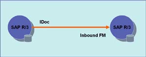 Data from custom tables (created in customer namespace) is to be formatted into an IDoc and sent from one SAP R/3 system to another using ALE service. We need to have two instances of SAP R/3 systems or we can simulate this on two clients of the same SAP R/3 system.
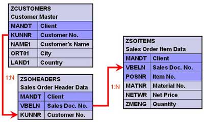
Create three tables as shown below.
Creating Custom IDoc type and Message type
All the objects created should be present on both source as well as target system(s).
1. Create segments – Transaction WE31
- Create a segment ZRZSEG1
- Add all fields of table ZCUSTOMERS to it
- Save the segment
- Release it using the menu path Edit -> Set Release
- Similarly create two more segments given below
- Seg. ZRZSEG2 – to hold all fields of table ZSOHEADERS
- Seg. ZRZSEG3 – to hold all fields of table ZSOITEMS
2. Create Basic IDoc type – Transaction WE30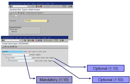
- Create a Basic type ZRZORDER
- Add the created segments in the hierarchy shown
- Maintain attributes for each of the segments
- Save the object and go back
- Release the object using the menu path Edit -> Set Release
3. Create/Assign Message type – Transactions WE81/WE82
- Go to WE81
- Create a new Message type ZRZSO_MT
- Save the object
- Go to WE82 and create new entry
- Assign the message type ZRZSO_MT to the basic type ZRZORDER
- Also specify the Release Version
- Save the object
Thus we have defined the IDoc structure which will hold the data to be transferred. In the next part of the article we will understand the outbound settings, i.e. the settings to be done in the source system.
Beginner’s Guide to ALE and IDocs - Part II
January 20th, 2008 Riyaz
Tiny link: (useful for email) http://www.riyaz.net/?p=19
In the previous part we created an IDoc structure which can carry our data from source system to target system(s). In this part we will understand how to setup the source system to be able to generate and send an outbound IDoc.
Outbound Settings
Define Logical Systems and Assign Client to Logical System – Transaction SALE
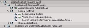
- Go to Define Logical System (See the figure)
- Define a new logical system to identify the local system and save it
- Now, go to Assign Client to Logical System (See the figure)
- Add a new entry
- Specify the client, previously created logical system and other attributes
- Save the entry
- Define a new logical system to identify the partner system and save it
Maintain RFC Destinations – Transaction SM59
- Create a new RFC destination for R/3 type connection
- Specify the target host on Technical settings tab
- Provide the Logon credentials on the Logon/Security tab
- Save the settings
- To verify the settings, Click on Test connection or Remote logon
Define Ports – Transaction WE21
- We need to define a tRFC port for the partner system
- Click on Transactional RFC node
- Create a new port
- Provide a description
- Specify the name of the target RFC destination
- Save the object
Maintain Distribution Model – Transaction BD64
- Click on Change
- Create a new model view
- Provide a Short text and Technical name to the model view
- Add message type
- Specify sender and receiver systems
- Also, specify the message type that we created previously
- Save the Distribution model
Generate/Create Partner Profile – Transactions BD82/WE20
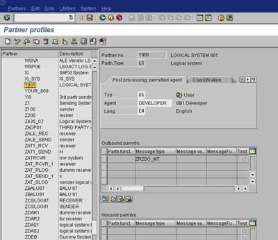
- To generate Partner profiles automatically you may use BD82 or go to BD64 and use the menu path Environment -> Generate partner profiles
- Otherwise, you may use transaction WE20 to create a partner profile
- On selection screen, specify the model view, target system and execute
- The result log will be displayed on the next screen
- To verify the partner profile go to WE20
- Check the partner profile for the target system
Distribute Model View – Transaction BD64
- Select the Model View
- Go to menu path Edit -> Model View -> Distribute
- Result log will be displayed on the next screen
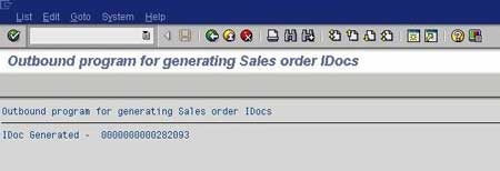
Outbound IDoc Generation Program
Create an executable program ZRZ_ORDER_IDOC in SE38. Below, I have described the program logic:
- Fetch the data from the DDic tables ZCUSTOMERS, ZSOHEADERS and ZSOITEMS as per the selection criteria
- Fill the control record structure of type EDIDC
- Specify message type, Basic IDoc type, tRFC Port, Partner number and Partner type of the receiver
- Fill the data records
- Define structures like the IDoc segments
- Fill the structures with fetched data
- Pass the segment name and the above structure to the appropriate fields of EDIDD type structure
- Append the EDIDD structure to the EDIDD type internal table
- Now, call the function module MASTER_IDOC_DISTRIBUTE and pass the IDoc control record structure and data record table
- Commit work if return code is zero
- Function module returns a table of type EDIDC to provide the details about generated IDoc
- Display appropriate log
You can download sample code for the above program here.
Thus we have completed sender side configuration required for ALE. In the next part we will see how to configure the receiving system to be able to receive and post the inbound IDoc.
Beginner’s Guide to ALE and IDocs - Part III
In the previous parts we learned how to create a custom IDoc and set up the source system to send an outbound IDoc. In this part we will learn how to configure the receiving SAP R/3 system to be able to receive and post the inbound IDoc.
Inbound IDoc Posting Function Module
In the receiving system, create a function module Z_IDOC_INPUT_ZRZSO_MT using SE37. Below, I have described the logic for the same.
Add Include MBDCONWF. This include contains predefined ALE constants.
Loop at EDIDC table
- Check if the message type is ZRZORDER. Otherwise raise WRONG_FUNCTION_CALLED exception
- Loop at EDIDD table
- Append data from the segments to appropriate internal tables
- For example: append data from ZRZSEG1 segment to the internal table of type ZCUSTOMERS
- Update the DDic tables from internal tables
- Depending on the result of the update, fill the IDoc status record (type BDIDOCSTAT) and append it to the corresponding table.
- Status 53 => Success
- Status 51 => Error
You can download the sample ABAP code for the above function module here.
Inbound Settings
- Define Logical Systems – Transaction SALE (Please refer to Outbound Settings discussed in previous part)
- Assign Client to Logical System – Transaction SALE (Please refer to Outbound Settings discussed in previous part)
- Maintain RFC Destinations – Transaction SM59 (Please refer to Outbound Settings discussed in previous part)
- Define Ports – Transaction WE21 (Please refer to Outbound Settings discussed in previous part)
- Generate/Create Partner Profile – Transactions BD82/WE20 (Please refer to Outbound Settings discussed in previous part)
- Assign Function Module to Logical message – Transaction WE57
- Create a new entry
- Specify name of the Function Module as Z_IDOC_INPUT_ZRZSO_MT
- Also, specify Type as F, Basic IDoc type as ZRZORDER, Message type as ZRZSO_MT and Direction as 2 (Inbound)
- Save the entry
- Define Input method for Inbound Function Module – Transaction BD51
- Create a new entry
- Provide Function Module name as Z_IDOC_INPUT_ZRZSO_MT
- Specify the Input method as 2
- Save the entry
- Create a Process Code – Transaction WE42
- Create a new Process Code ZPCRZ
- Select Processing with ALE Service
- Choose Processing type as Processing by function module
- Save the entry
- On the next screen, select your function module from the list
- Save the changes
- Now you will be taken to the next screen
- Double-click on Logical message
- In the Assignment to logical message, specify the message type ZRZSO_MT
- Save the changes
Send and receive data
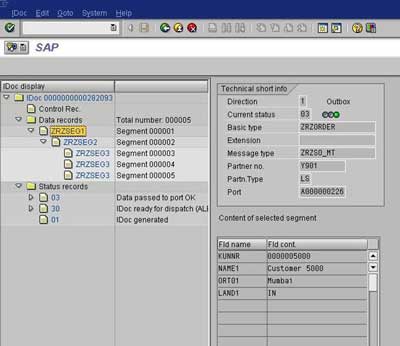
On the sender system, execute the IDoc Generation Program. Check the status of IDoc using transaction WE02.
Check the status of the IDoc in the receiver system using transaction WE02. You can also check the contents of DDic tables to make sure that the records have been created in the receiver system.
Thus to summarize we have learned how to:
- Create a custom IDoc
- Write an Outbound IDoc Generation Program
- Write Inbound Function Module to post Inbound IDoc
- Configure and test ALE scenario to transmit data between systems distributed across the network
Subscribe to:
Posts (Atom)